The simplifying language: Topology
Constructions involving numerous quantifiers are different to grasp. A good theory splits such constructions introducing appropriate notions and building a suitable language. Let  be a subset in the Euclidean space and
  a metric on it which we (only for simplicity!) will assume translation invariant and denote
  . Everywhere below
  will denote the open ball of radius
  centered at a point
  :
:  .
.
Definitions. A point  is called interior point, if
  such that the open ball
  lies in
  , i.e.,
  . This is the same as saying that
  .
.
A point  is called exterior point, if it is interior for the complement
  . The points that are neither interior nor exterior are called the boundary points of .
The sets of all interior and boundary points of are denoted  and
and  respectively.
A point  is called an accumulation point (for ), if
  such that
  . The set of all accumulation points for is called its closure and denoted by
  . Sometimes the notation
  is used for the closure.
Exercise. Prove that  . Prove that the exterior of is
  .
.
Exercise. Prove that the notions of interior, exterior and boundary do not depend on the choice of the distance function in  .
.
Definitions. A subset  is called open, if it coincides with its own interior,
  . The subset is closed, if it coincides with its own closure
  .
.
Exercise. Assume that  and
and  . Describe interior, closure and boundary of this segment. Is it open? closed? neither?
Exercise. Show that the complement of an open subset is closed and vice versa, the complement of a closed subset is open. Show that Are there other subsets that are both open and closed?
Theorem 1.
 and
and  are both open and closed simultaneously.
 - Union of any family (infinite or even uncountable) of open sets is open.
- Finite intersection of open sets is open.
- Intersection of any Union of any family (infinite or even uncountable) of closed sets is closed.
- Finite union of closed sets is closed.
Continuity as a topological notion
Consider first the case of maps (functions) defined on the entire Euclidean space,  .
.
Temporary Defininion. A map as above will be called an O-map1, if the preimage of any open set  is an open subset
  .
.
Lemma 1. A map  continuous at all points of , is an O-map.
Proof. Consider any open set  and its preimage
  . Let
. Let  be any point in this preimage: by definition, this means that
  . Since
  is open in
  , there exists a ball
  of positive radius
  which lies in . By continuity of at
  , there exists
  such that
  , that is, all points of the ball
  are mapped inside , hence inside . Therefore the preimage
  together with the point contains a small ball around , that is, is an interior point for
  . Since was chosen arbitrarily, this means that all points of are interior points, hence is open. Since was chosen arbitrary, we have proved that is an O-map. Q.E.D.
Lemma 2. An O-map is continuous at every point .
Proof. Let be an arbitrary point, and denote  . Consider an arbitrary open ball
  of positive radius . To prove the continuity of , we need to find an open ball around such that its -image is inside . But since is open2, its preimage is also open in by the definition of an O-map applied to . The openness of means that each its point, in particular, the point , is interior for and hence the ball with the required property exists. Q.E.D.
These two lemmas together prove that at least for maps whose domain is the entire Euclidean space, the property “Preimages of open sets are open” (as stated in the Temporary Definition) is fully equivalent to the property of being continuous on the entire domain.
How this result should be modified for maps  whose domains are only proper subsets of the Euclidean subspace, ? The answer is simpler than you might imagine. You don’t need to modify the definition of O-maps, you need to twist the definition of open sets, making it relative to the arbitrary domain of definition of the map .
Definition. Let be an arbitrary (not necessarily open) subset of the Euclidean space. A subset  is called open relative to , if there exists an open (in the original sense) subset
  such that
  .
.
One can immediately and easily check (by just passing from open sets to relatively open obtained by intersection with any subset , that:
- Theorem 1 above remains valid in the relative sense, with the only required correction that the “absolute” should replace as a set which is both relatively open and relatively closed.
- The proofs of both Lemmas 1 and 2 remain literally true if we replace the (ordinary, absolute) openness by the openness relative to : indeed, for
 the value
  is simply undefined hence cannot violate any inequality or inclusion.
As a result, we obtain the following reformulation of continuity for maps defined on proper subsets of the Euclidean space.
Theorem 2. A map  defined on a subset is continuous on its domain of definition, if and only if the preimage
  of any open subset is an open subset relative to .
Note that this equivalent definition of continuity of a map at all points of its domain formally requires only one quantifier, assuming that the notion of an open set is sufficiently familiar to the reader: indeed, it asserts that is continuous if and only if

But there is much more to gain from the topological approach.
Topological spaces
The topological language that we introduces in a very particular settings (for subsets of the Euclidean sets) actually works in a much broader context. Indeed, Theorem 1 above is a pretty good motivation for the following definition.
Definition. A topological space  is an abstract set (eventually very large, much larger than subsets of such that some of its subsets are distinguished by bearing a noble name of open sets
  . There are only three axioms these open sets must obey:
- The total space itself and the empty set
 are open.
- Union of any number of open sets is again open.
- Intersection of any finite number of open sets is open.
Note that the axioms do not specify any way concrete way how open sets should be defined in any concrete example. Only their algebraic properties in the Boolean algebra are important. This is dangerous (examples may challenge our intuition) but provides great versatility. In particular, Theorem 2 above allows to define the continuity for any map  between any two topological spaces, with an immediate trivial corollary that composition of any two continuous maps (when defined) will again be continuous. This becomes a trivial observation (why?), although the proof in the “classical” case is also very easy.
What we (on our rather down-to-earth) level can gain from so abstract constructions? Quite a lot, even if we consider only topological spaces embedded in with the supply of open spaces through the definition of relative openness.
Connected spaces
Using only topological terms, we can formulate one of the most basic properties of sets, the fact that they do not fall apart as unions of smaller sets. It is instrumental in the study: if something is built from smaller components that do not interact with each other, then one can study these components separately and then “mechanically” bring the results together.
Definition. A topological space is called disconnected (or disconnect), if it can be represented as a disjoint union of two open sets,  with
with  . If such representation is impossible, we call the space connected. Examples are numerous: the Euclidean spaces of all (finite) dimensions are connected, yet the set
 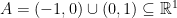 is disconnected, as the two relatively open subsets provide the partition.
Remark. The property of connectedness is very closely related to the completeness of the real numbers. One can consider the rational numbers  as a topological space and define open and closed sets relative to them. Then the sets
  and
and  are obviously (relatively) open and disjoint from each other, but their union is the whole of .
Theorem 3. A continuous map preserves connectedness: if is connected, then so is  .
.
Proof. Assume that  are two disjoint open subsets such that
  . Then their preimages
  and are open by continuity of , obviously disjoint and their union gives in contradiction with the assumption on . Q.E.D.
Exercise. Describe subsets of  which are connected topological spaces with respect to the relative topology inherited from . Derive from Theorem 4 the familiar Theorem on intermediate value: if a function continuous on a segment
  (finite or infinite, doesn’t matter) takes two different values
  , then it takes also all intermediate values
 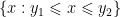 .
.
Warning. One should be very careful and never confuse between preimages and images. The preimage of the connected interval  by the continuous map
  ,
,  , is the disconnected union
 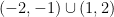 .
.
Another example of a useful notion that is of purely topological nature, is that of an isolated point.
Definition. A point  is an isolated point of a topological space (e.g., a subset with the topology defined by the relatively open sets), if the one-point subset
  is both open and closed3.
Proposition. Any map is automatically continuous at all isolated points of . Q.E.D.
Compact sets
Another purely topological property of topological spaces (in particular, subsets of with the inherited relative topology) is a mighty generalization of some finiteness property. Recall that finite collections (say, of positive numbers) allow to choose a minimal element, which will still be positive: infinite collections of positive numbers, like the set 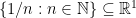 do not allow such choice: the only nonnegative element that is smaller than all number in the above set, is zero which is non-positive.
Definition. A collection (finite or infinite) of sets  is an open covering of the topological space , if:
- All sets
 are open, and
 .
.
When dealing with subsets of Euclidean spaces we can assume that a covering  is a collection of open subsets
  in , which contain in their union,
  .
.
A subcovering is a subcollection 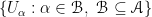 , that is, a collection of open sets which still cover obtained by rarefying
  , that is, discarding (throwing away) some open sets from the initial covering.
Example. Let  is a function continuous at all points of its domain. Then for every point there exists an open set
  such that
 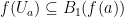 . The collection
  is an open covering of . Another example of the covering is the representation of the real line as the union of open sets,
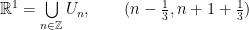 .
.
The second covering is minimal in the sense that removing of any of the sets  is not covering of anymore: the middle third of the corresponding segment
 ![[n,n+1]](https://s0.wp.com/latex.php?latex=%5Bn%2Cn%2B1%5D&bg=ffffff&fg=000000&s=0&c=20201002) will become uncovered. Yet some of the coverings are definitely non-minimal, and one can safely remove some of the open sets which were used to cover.
will become uncovered. Yet some of the coverings are definitely non-minimal, and one can safely remove some of the open sets which were used to cover.
Definition. A topological space (i.e., a set with the inherited topology) is called compact, if any open covering can be decimated to produce a finite open subcovering.
Make no mistake: compactness does not mean that there simply exists finite open covering: any subset can be covered by just one open set (e.g., the space itself). Compactness means that a finite covering can be achieved by discarding all but finitely many open sets from any open covering. This definition is rather technical, it is somewhat difficult to digest (people rarely have any working intuition with coverings and their finite subcoverings), yet the idea is quite transparent: compact sets possess some hidden “finiteness”. Yet in a very surprising way sometimes compactness can be achieved by adding some points to a non-compact spaces. For instance, the non-compact real interval  (it is non-compact because the infinite open covering
  cannot be reduced to a finite subcovering) can be compactified by adding two endpoints
  and
and  . The explanation “on one leg” of this phenomenon is simple: adding the extra points imposes additional requirement on the collection of open sets to be a covering, i.e., to cover the extra point as well.
Exercise. An unbounded set cannot be finite. Indeed, consider the union of all open balls of radius 1 around all points of ,  . This is a covering, since each point belongs to “its” ball. Yet no finite subcovering can be selected from this covering: the union of finitely many balls of radius 1 must be bounded. A similar easy argument shows that a set which is not closed, also cannot be compact.
Proposition. The real closed segment ![[0,1]\subseteq\mathbb R^1](https://s0.wp.com/latex.php?latex=%5B0%2C1%5D%5Csubseteq%5Cmathbb+R%5E1&bg=ffffff&fg=000000&s=0&c=20201002) is compact.
is compact.
Proof. Consider an arbitrary open covering  and let
 ![M\subseteq [0,1]](https://s0.wp.com/latex.php?latex=M%5Csubseteq+%5B0%2C1%5D&bg=ffffff&fg=000000&s=0&c=20201002) be the set of all points
be the set of all points ![a\in[0,1]](https://s0.wp.com/latex.php?latex=a%5Cin%5B0%2C1%5D&bg=ffffff&fg=000000&s=0&c=20201002) such that the subsegment
such that the subsegment ![[0,a]](https://s0.wp.com/latex.php?latex=%5B0%2Ca%5D&bg=ffffff&fg=000000&s=0&c=20201002) admits a finite subcovering selected from . Since
admits a finite subcovering selected from . Since  is covered, the set
  contains some positive number. Denote by
  the supremum of points in ,
  . We claim that
  . Indeed, if
  , then
  for some open set
  . But since is open, for some sufficiently small the point
  would still be in and hence the same finite subcovering will still “serve” the point . This contradicts our choice of as the exact supremum. This leaves the only possibility that , that is, the entire segment
 ![[0,1]](https://s0.wp.com/latex.php?latex=%5B0%2C1%5D&bg=ffffff&fg=000000&s=0&c=20201002) admits a finite subcovering selectable from . Q.E.D.
admits a finite subcovering selectable from . Q.E.D.
Remark. Compactness of the closed segment uses the fact that any bounded set set of real numbers has the exact supremum. Indeed, the “rational closed segment  is not compact. To see this, let us enumerate all points of
  by natural numbers,
  (this is possible, since is countable!) and consider the open covering which covers each point
  by the interval (open ball) of radius
  centered at this point. This infinite covering does not admit a finite subcovering of , since the sum of lengths of any finite number of intervals from is less than
  which is less than
  , so at least one point of will remain “unserved”.
Compactness and continuity
Let  be topological spaces and a continuous map.
Theorem. If is compact, then its image is  is compact in .
Proof. Let  be an arbitrary open covering of . Consider the sets
  . By continuity of , these sets are open and together give a covering $\mathscr U$ of . Since is assumed compact, there exists a finite subcovering of . The corresponding finitely many sets
  give a finite covering of . Q.E.D.
Combining this Theorem with the Exercise above, we see that any continuous function is bounded on any compact topological space. Note that the preimage of a compact set may well be noncompact (consider any constant function on  ).
).
Problem. Prove that any closed subset of a compact topological space is also compact.
The following result, which we will not prove, describes all compact subsets of finite-dimensional Euclidean space.
Theorem. A subset is compact, if and only if it is bounded (i.e.,  ) and closed (
 ). Q.E.D.
Warning
The simplicity obtained by carefully crafting the definitions may well be misleading. Open and closed subsets of provide a rich basis for our finitely-dimensional intuition. Yet the general notion of a topological space without assuming that its topology is inherited from an embedding of in some space (recall that by “topology” we mean a rule that allows to declare some subsets of open) allows for some surprising results.
Example. Consider the real line with the origin deleted, but with two distinct imaginary points  added instead. We can introduce a “perverse topology” on this set
  by declaring that the open sets are the open sets in the former by replacing by only one of the two artificially created points . This rule describes all open subsets of
  which (check it at home) are consistent with claiming that
  is a topological space.
What is “wrong” with this space? The answer is very easy: the two distinct points,  and
and  , cannot be separated by disjoint open sets: any two sets
  open in the topology of and containing the points and respectively, necessarily intersect:
  . This means that the topology of cannot be generated by any distance function on . This is an example of the so called non-Hausdorff topology: it happens quite often when dealing with the topological spaces of algebraic origin.
Example. The same space $\mathbb R^1$ can be equipped with a non-standard topology, the so called Zariski topology: namely, declare closed only finite sets and (and the line itself). Hence open will be complements to finite point sets (and the empty set). This topology is also non-Hausdorff: any two non-empty open sets intersect.
Footnotes
 of two close points
  in the domain are close to each other in the target space of a function
  at a point
  ) is nothing more than the possibility of extending the “natural” domain of this function (given, say, by an explicit function) by assigning the value
  so that the extended function retains continuity on the larger set
  . Usually such procedure is used to “avoid” division by zero in the expressions like
  on the diagonal
  or
or  at the origin, that will appear when introducing derivatives later.
  : the closer a point
  approaches
  . Of course, this completely transparent phrase of a human language requires quantifiers to measure “proximity” and “smallness” and how one implies the other.
  is a set
  , a binary commutative invertible operation (making
  .
.  between two (in general, different) vector spaces is called linear, if it “respects” both linear operations. In particular, it must map the zero vector of
  . If
. If  , then all linear functions have a simplest form
  for some number
  (possibly, zero), in the general multidimensional case a linear map is determined by
  real numbers which are naturally arranged in the form of a matrix, an
  -table.
  , is not linear (
 unless
  , in which case the shift becomes a dull identical map). Thus we need to make one last step and consider the smallest class of maps that would contain all linear maps and all shifts (parallel translations) and closed by compositions. This class is called the class of affine maps: reducing similar terms, one can show that by definition, an affine map
  is a composition,
  , where
  is a linear map and $T$ a translation in the target space. Explicitly, we have
  (“linear non-homogeneous function”). Note that there is a well-established tradition not to enclose the argument of linear maps in the parentheses and write
  rather than
  : this is because one can treat
  (functions of one real variable). If
 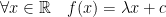 for some two constants
  , which could be found using the values of
  at any two different points
  by the formulas
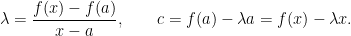
 do not depend on the choice of the two points
  .
.  there exists the limit
 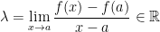 . Then the function
  , in the following sense: the relative error of approximation
 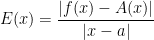 tends to zero as
  ,
,  .
.  is called the derivative of
  the differential of
  . If
. If  ), while the differential will become a function of two independent arguments
  (usually denoted by
  without extra braces, or simply
  , omitting both arguments.
 .
.  and taking values in another space
  is “too narrow” to talk in proper geometric terms.
  sufficiently close to each other, their images
  and $b=f(a)$ in
  . This function should be far from arbitrary:
  for any pair of points; the distance is zero if and only if the two points coincide,
  , that is, the distance is a symmetric function;
 we have
 satisfies all these axioms. (Don’t think that this is the only function with such properties! The function
  also satisfies all of them.) Yet in
  there is a whole family of distance functions,
 ![\textrm{dist}(x,y)=\sqrt[p]{\sum_{i=1}^n(x_i-y_i)^p}](https://s0.wp.com/latex.php?latex=%5Ctextrm%7Bdist%7D%28x%2Cy%29%3D%5Csqrt%5Bp%5D%7B%5Csum_%7Bi%3D1%7D%5En%28x_i-y_i%29%5Ep%7D&bg=ffffff&fg=000000&s=0&c=20201002) for any positive
for any positive  . The case
  appears as the limit case when
  grows to infinity, the case
  corresponds to the usual Euclidean metric.
  we will call open balls centered at
  for any of the above distance functions on
  for all
  (invariance by translations). Not all functions satisfying the above three properties possess this invariance.
  .
.  is trivially valid for any function and the axiom of distance! Besides, it is not clear, for which pairs
  this claim must hold.
 can be called
  -small, if
  -small, with two positive numbers
  , getting the implication
 .
. that involves four “free variables”,
  . What shall we do with them? There are two options, either to tie down each variable by one of the two quantifiers $\forall, exists$ or to designate them as a “parameter” that has to be specified in advance.
  . They clearly play a symmetric role, so it would be natural to assign the same quantifier in front of each of them, and this quantifier is obviously “for all”,
  (warning: see below). As for the two remaining “scale variables”
  , we can play around with the two quantifiers
  and
and  , where
  are independently either
  or
or  , and placed in a different order: altogether this yields 8 various possible combinations (some of them identical).
  .
. -closeness (resp.,
  in the target space one can find the proximity measure
  in the domain such that for any two
  are
are  . Then if
  , then for any fixed
  will eventually exceed any given
  is large enough, so the quadratic function, the nicest of all nonlinear function, turns out to be not uniformly continuous on its natural domain. This happens because the natural domain
  .
. and considering it as a parameter. The corresponding definition (stripped of the word “uniformly“, looks as follows.
  such that
  its image
  ,
,  .
.  that depends on two logical “free variables”
 converges” takes the form involving the horrible four (!) quantifiers:
 , where the claim
  , involving the number
  of the unit circle or the
  , where
  is the solution of the simplest differential equation
  with the initial condition
  .
. with rational left and right bounds
  . Of course, we have to assume that the system of inequalities is self-consistent and defines not more than one “number”. Consistency means that all left bounds are not exceeding any right bound and vice versa. Uniqueness requires (at least!) that no two different rational numbers satisfy all inequalities forming the system. Obviously, any rational number
  satisfies the trivial inequality
  , so the “new” numbers will automatically include all “old” rational numbers.
 , such that
  and
and  consists of at most one point. Any such partition (called the Dedekind cut) is intuitively associated with a “number”
  .
. (because the inequalities will be inverted if multiplied by the negative number), then we easily define subtraction as addition of
  . Some technical efforts are required to define product and ratio of numbers in
  (with or without zero), we can try and extend this number system to add some “missing elements”. These missing elements are required to solve the equations that have no natural solutions. Two special cases of examples are most important: those of the form
  with
with  and
and  and those of the form
  with
with  depending on interrelations between the integer coefficients. His way of presenting these rules was much later named after him by the word “algorithm” which now stands for any deterministic rule of performing manipulations.
 does not have rational solutions, while geometrically the expected solution is yielded by the diagonal of the unit square. The Greeks turned to the geometric constructions by ruler and compass as the “source” for legally accepted numbers. Today the class of such numbers is called the class of \emph{quadratic irrationals}. These quadratic irrationals, however, are not sufficient to solve the three famous problems, duplication of the cube, trisection of the angle and squaring the circle.
 can be constructed as the set of formal expressions
  with
with  closed by all arithmetic operations. This set can be ordered by an order
  compatible with the arithmetic operations, assuming that
  .
. (also absent over the rationals): to that end, we consider all expressions of the form
  and show that it is closed by all arithmetic operations assuming that
  . However, unlike in the previous case, the set
  is a field that cannot be ordered.
 must remain unsolvable unless we agree to say good bye to the laws of arithmetic. One needs a special motivation and very special constellation of properties to make this process available.
